Example: Tim Churches

The following code is modeled after an illustration designed for RPy done by Tim Churches (RPy website). The code analyzes data on the Old Faithful geyser in Yellowstone National Park. The code illustrates the ease and power of RinRuby and its methods. The RinRuby code is shown on the left and the original RPy code on the right.

require "rinruby"

faithful_data = {"eruption_duration"=>[], "waiting_time"=>[]}

for row in File.readlines('faithful.dat')[1..-1]
splitrow = row.chomp.split
faithful_data["eruption_duration"] << splitrow[0].to_f
faithful_data["waiting_time"] << splitrow[1].to_i
end

R.ed = faithful_data["eruption_duration"]
R.eval "edsummary <- summary(ed)"
edsummary = R.pull("as.vector(edsummary)")
keys = R.pull("names(edsummary)")
puts "Summary of Old Faithful eruption duration data"
keys.each_index do |i|
puts "#{keys[i]}: #{sprintf('%.3f',edsummary[i])}"
end
puts
puts "Stem-and-leaf plot of Old Faithful eruption duration data"
R.eval "stem(ed)"

R.eval <<EOF
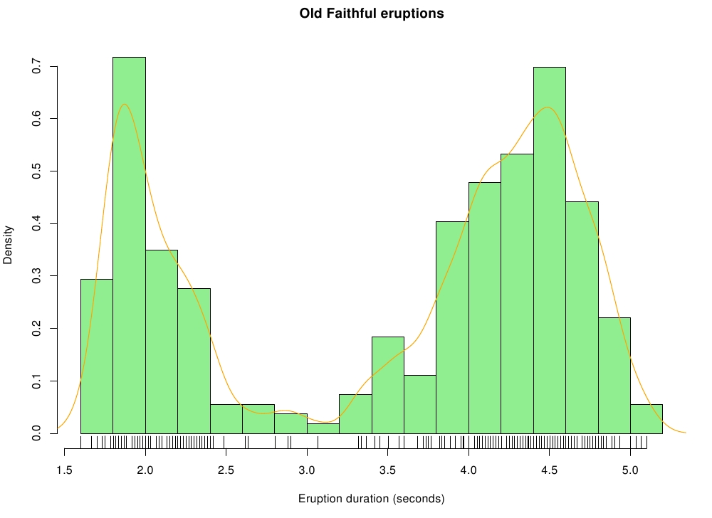
png("faithful_histogram.png",width=10,height=7.5)
hist(ed,seq(1.6, 5.2, 0.2), prob=1,col="lightgreen",
main="Old Faithful eruptions",xlab="Eruption duration (seconds)")
lines(density(ed,bw=0.1),col="orange")
rug(ed)
dev.off()
EOF

cutoff = 3
R.long_ed = R.ed.delete_if{ |x| x <= cutoff }
R.eval <<EOF
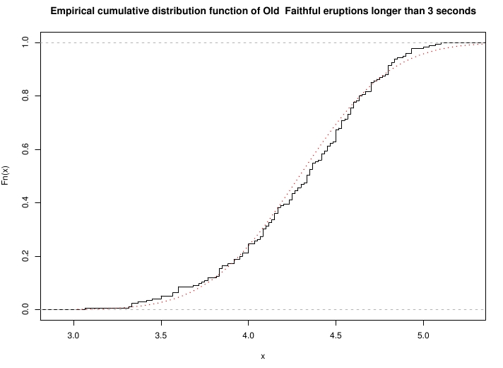
png('faithful_ecdf.png',width=10,height=7.5)
# library(stepfun)           # package has been merged into 'stats'
plot(ecdf(long_ed), do.points=0, verticals=1,
      main=paste('Empirical cumulative distribution function of Old',
                 ' Faithful eruptions longer than #{cutoff} seconds'))
x <- seq(3,5.4,0.01)
lines(seq(3,5.4,0.01),pnorm(seq(3,5.4,0.01),mean=mean(long_ed),
       sd=sqrt(var(long_ed))), lty=3, lwd=2, col='red')
dev.off()

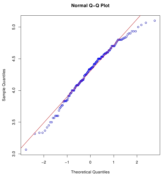
png('faithful_qq.png',width=10,height=7.5)
par(pty="s")
qqnorm(long_ed,col="blue")
qqline(long_ed,col="red")
dev.off()
EOF

# R.eval "library('ctest')" # package has been merged into 'stats'
puts
puts "Shapiro-Wilks normality test of Old Faithful eruptions" +
" longer than #{cutoff} seconds"
R.eval "sw <- shapiro.test(long_ed)"
puts "W = #{sprintf("%.4f",R.pull("sw$statistic"))}"
puts "p-value = #{sprintf("%.5f",R.pull("sw$p.value"))}"

puts
puts "One-sample Kolmogorov-Smirnov test of Old Faithful eruptions" +
" longer than #{cutoff} seconds"
R.eval "ks <- ks.test(long_ed,'pnorm',mean=mean(long_ed),"+
"sd=sqrt(var(long_ed)))"
puts "D = #{sprintf("%.4f",R.pull("ks$statistic"))}"
puts "p-value = #{sprintf("%.4f",R.pull("ks$p.value"))}"
puts "Alternative hypothesis: #{R.pull("ks$alternative")}"
puts

from rpy import *

faithful_data = {"eruption_duration":[],
"waiting_time":[]}

f = open('faithful.dat','r')

for row in f.readlines()[1:]: # skip the column header line
    splitrow = row[:-1].split(" ")
    faithful_data["eruption_duration"].append(float(splitrow[0]))
    faithful_data["waiting_time"].append(int(splitrow[1]))

f.close()

ed = faithful_data["eruption_duration"]
edsummary = r.summary(ed)
print "Summary of Old Faithful eruption duration data"
for k in edsummary.keys():
print k + ": %.3f" % edsummary[k]
print
print "Stem-and-leaf plot of Old Faithful eruption duration data"
print r.stem(ed)

r.png('faithful_histogram.png',width=733,height=550)
r.hist(ed,r.seq(1.6, 5.2, 0.2), prob=1,col="lightgreen",
main="Old Faithful eruptions",xlab="Eruption duration (seconds)")
r.lines(r.density(ed,bw=0.1),col="orange")
r.rug(ed)
r.dev_off()

long_ed = filter(lambda x: x > 3, ed)
r.png('faithful_ecdf.png',width=733,height=550)
r.library('stepfun')
r.plot(r.ecdf(long_ed), do_points=0, verticals=1, col="blue",
       main=paste("Empirical cumulative distribution function",
                  " of Old Faithful eruptions longer than 3 seconds")
x = r.seq(3,5.4,0.01)
r.lines(r.seq(3,5.4,0.01),r.pnorm(r.seq(3,5.4,0.01),mean=r.mean(long_ed),
        sd=r.sqrt(r.var(long_ed))), lty=3, lwd=2, col="red")
r.dev_off()

r.png('faithful_qq.png',width=733,height=550)
r.par(pty="s")
r.qqnorm(long_ed,col="blue")
r.qqline(long_ed,col="red")
r.dev_off()

r.library('ctest')
print
print("Shapiro-Wilks normality test of Old Faithful eruptions" +\
" longer than 3 seconds")
sw = r.shapiro_test(long_ed)
print "W = %.4f" % sw['statistic']['W']
print "p-value = %.5f" % sw['p.value']

print
print("One-sample Kolmogorov-Smirnov test of Old Faithful eruptions" +\
" longer than 3 seconds"
ks = r.ks_test(long_ed,"pnorm", mean=r.mean(long_ed),
sd=r.sqrt(r.var(long_ed)))
print "D = %.4f" % ks['statistic']['D']
print "p-value = %.4f" % ks['p.value']
print "Alternative hypothesis: %s" % ks['alternative']
print

Output:

The output from both scripts is the same, except that RinRuby maintains the order of the summary statistics while RPy changes the order. The output shown below is from RinRuby.

Summary of Old Faithful eruption duration data
Min.: 1.600
1st Qu.: 2.163
Median: 4.000
Mean: 3.488
3rd Qu.: 4.454
Max.: 5.100

Stem-and-leaf plot of Old Faithful eruption duration data

The decimal point is 1 digit(s) to the left of the |

16 | 070355555588
18 | 000022233333335577777777888822335777888
20 | 00002223378800035778
22 | 0002335578023578
24 | 00228
26 | 23
28 | 080
30 | 7
32 | 2337
34 | 250077
36 | 0000823577
38 | 2333335582225577
40 | 0000003357788888002233555577778
42 | 03335555778800233333555577778
44 | 02222335557780000000023333357778888
46 | 0000233357700000023578
48 | 00000022335800333
50 | 0370

Shapiro-Wilks normality test of Old Faithful eruptions longer than 3 seconds
W = 0.9793
p-value = 0.01052

One-sample Kolmogorov-Smirnov test of Old Faithful eruptions longer than 3 seconds
D = 0.0661
p-value = 0.4284
Alternative hypothesis: two-sided